- Available in Composites Engineering
Design (CPE) and Composites Design for Manufacturing
(CPM).
- Some Propagation modes, Deformation options, Simulation: Advanced Parameters, and Analysis: Advanced Parameters are available only if Composites Fiber Modeling (CFM) is available. See details below.
- In a few cases, the position of seed points may lead to an invalid rosette transfer and incorrect fiber directions. The problem is detected as you click Preview, and a warning is displayed.
- A check for overlap helps you understand that too much fabric is present in an area, requiring a cut out or dart.
- Producibility parameters (i.e. seed point, warp and weft) are stored as
Producibility params.x under each ply,
and may be later used when flattening plies.
Existing producibility parameters sets are kept.
Go to Tools > Options > Mechanical Design > Composites Design to define the Producibility default behavior.
Start the Producibility for Hand Layup
-
Click Producibility for Hand Layup
 in the Flattening toolbar.
The Producibility for Hand Layup dialog box opens. -
Select the Propagation type from the list.
- If Composites Fiber Modeling is not available,
proposed types are:
- Minimum distortion
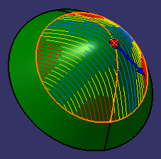
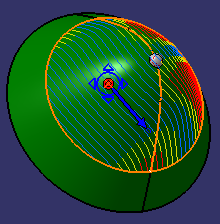
In the above picture, the shape of the surface is not symmetrical.
On this non-symmetrical shape, the fiber propagation with the Minimum Distortion option follows
the curvatures of the surface while minimizing the deformation of the fibers. - Symmetric
With the Symmetric option, the system forces the fiber propagation to be symmetrical.
- Minimum distortion
- If Composites Fiber Modeling is available, proposed
types are:
- Minimum distortion
- Symmetric
- CFM Optimized Energy
- CFM Optimized MaxShear
- CFM Tape
- CFM UD Tape
- CFM Geodesic
- CFM FEFlatten
- CFM Energy (Frictionless).
See Propagation Type for more information.
- If Composites Fiber Modeling is not available,
proposed types are:
-
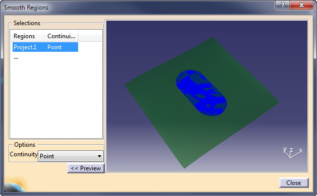
For any CFM propagation type, except CFM DEFlatten, define a Smooth Region.
- Select either a closed curve lying on the ply
surface, or a surface that intersects the ply surface,
resulting into a closed curve.
The curve provide the partition between a region of low strain and a region of high strain on the ply surface. - Right-click Smooth Regions to clear it.
- Click Edit to set continuity options for the
surface created from the selected curve.
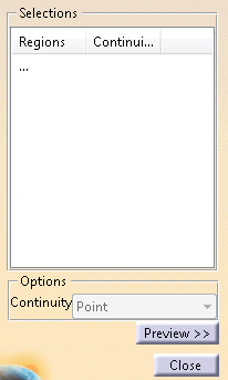
If you have selected a surface, continuity options are ignored. - Click Preview to inspect the smooth surface.
Preview is updated with continuity changes.
- Select either a closed curve lying on the ply
surface, or a surface that intersects the ply surface,
resulting into a closed curve.
-
If the seed point set at the geometrical center meets your needs, click Preview.
The fiber simulation is displayed.
Otherwise, select one of the other options. -
Select Selection from the list.
- Select an existing point.
The point is identified by a blue circle.
The fiber direction is displayed at this point.
- Click Preview.
The fiber simulation is displayed.
- Select an existing point.
-
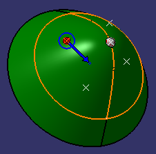
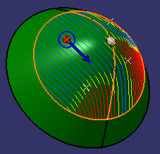
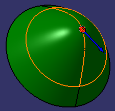
Select Indication from the list.
- Pick a point on the ply.
The point symbol is a circle. The fiber direction is displayed as a blue line.
- Click Preview.
The fiber simulation is displayed. The symbol of the point turns into a circle with handles.
- Drag the point to another location.
The simulation is updated dynamically, allowing you to select the best possible seed point location.
- Pick a point on the ply.
-
Alternatively, select Guide curves.
If the selected wireframe is open, it is recognized as a seed curve.
If it is closed, it is recognized as a region.
See Seed Curve and Order of Drape for more information.
See Creating a Rosette Transfer Curve to create one. -
Define the Mesh Step Length type (Scaled or Explicit).
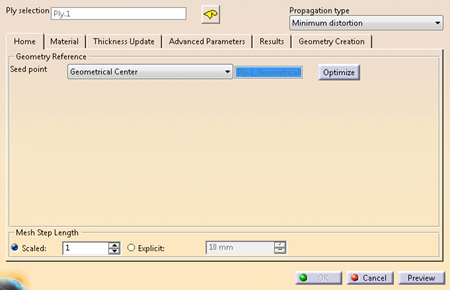
Optimize the Seed Point
For Composites producibility by layup of fabric over a curved surface,
the deformation of the fabric is highly influenced by the location of the
seed point of the draping process.
Optimize lets you optimize
the hand layup simulation by varying the seed point.
This optimization is done in iterations.
-
Still in the Home tab, click Optimize.
The Optimization dialog box opens.
-
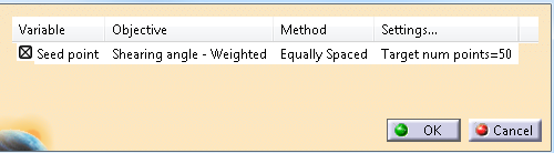
Activate and set up the optimization parameter: Seed point.
A contextual menu is available on each cell, with the possible following items: - For Objectives, possible values are:
- Shearing angle - Mean Absolute
- Shearing angle - Weighted
- Shearing angle - Greatest
- For Method, Equally Spaced is proposed, with a default number of 50 points over the ply surface.
- For Settings, the menu item is Edit, that opens a box to edit the number of points.
-
Click OK.
A progress bar is displayed with the following information:- Estimated number of iterations
- Completed iterations
- Completed time
- Mean time per iteration
- Estimated time remaining.
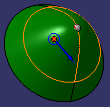
After simulations are run at each point, a marker of the appropriate color is displayed, corresponding to the maximum deformation and the allowed values. This provides a quick visualization of the best areas to begin draping.
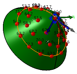
When the optimization is completed, the seed point is set to the optimum point.
Specify the Material Parameters
-
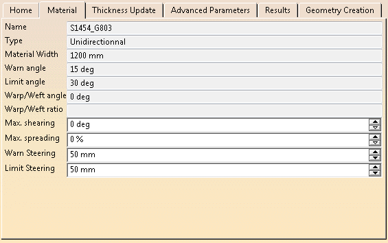
The following parameters are displayed for information and cannot be edited.- Name
- Type
- Material Width
- Warn angle
- Limit angle
- Warp/Weft angle
- Warp/Weft ratio
-
Edit the other parameters as necessary.
- Max. Shearing
- Max. Spreading
- Warn Steering
- Limit Steering
Update the Thickness
-
Go to the Thickness Update tab and select the With thickness update check box to activate it.
Note that the update processes the thickness provided for the material, not the effective one.

-
Press the required icon to define the type of computation.
- Constant Thickness
 :
With this option, the surface where the plies are drapped is
an offset (by the provided value) of the surface supporting
the plies. The plies ignore all ramps.
:
With this option, the surface where the plies are drapped is
an offset (by the provided value) of the surface supporting
the plies. The plies ignore all ramps. - Core Sampling
 :
With this option, the surface where the plies are drapped is
an exact elevated surface, computed from the core sample and
taking the ramps and drop off into account.
:
With this option, the surface where the plies are drapped is
an exact elevated surface, computed from the core sample and
taking the ramps and drop off into account.
The range field is the maximum thickness where plies will be querried by the core sampling operation.
Note that this option is more accurate but requests a more extensive computation. - User or Automatic Constant Offset
 :
With this option, the offset value is based on the plies
material thickness.
:
With this option, the offset value is based on the plies
material thickness.
- Constant Thickness
-
Select the elements to process, Full stacking or Ply group only.
-
When available, select Max Slope and enter a value.
Fine-Tune the Simulation
-
Go to the Advanced Parameters tab.
Its content varies with the type or propagation.
Minimum Distortion and Symmetric have no advanced parameters. -
For CFM Optimized Energy, Optimized MaxShear, Tape and UD Tape, set the Inadmissible Mode from the list, and enter a tolerance.
Both are described in Order of Drape. -
For FE Flatten,enter the parameters values.
See FE Flatten Propagation Mode for more information. -
When available, enter a small Free edge merge tolerance value (1.0e-3 or less), always in mm.
Fiber simulation is run on a high resolution mesh to closely match the surface geometry.
On very complex surfaces, subject to several operations, the meshes on the different surface patches do not merge completely, resulting in slits, and simulation errors.
A positive Free edge merge tolerance merges nodes on the free edges of the surface, removing the slits.
If Free edge merge tolerance is greater than the separation of any adjacent pair of free edge nodes, the value is automatically reduced to maintain the integrity of the mesh.
Manage the Results
-
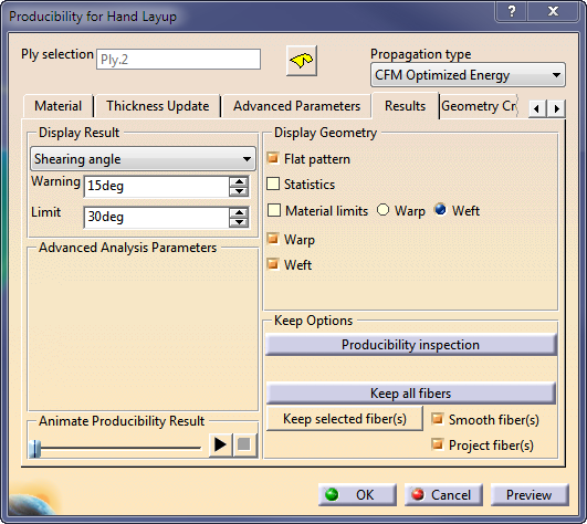
Go to the Results tab.
Not every result can be displayed on any geometry.
For example, it usually does not make sense to display the results on a flat pattern geometry. -
Click Preview to run the simulation.
-
Under Display Result, select the result to display from the list.
The content of the list, and other result options depend on the selected propagation type.
- For Symmetric
and Minimum distortion:
- Shearing angle
- Deviation
- Min tape length.
- For CFM Optimized Energy, CFM Optimized Max Shear,
CFM
Tape UD Tape:
- Shearing angle
- Sterring radius
- Deviation
- Min tape length.
- For CFM FE Flatten
- Shearing angle
- Deviation
- Min tape length
- Axial Strain.
- For Symmetric
and Minimum distortion:
-
For all results, enter the Warning and Limit values.
If those values exist in the material, they are proposed as default values.
If they do not exist in the material, they are proposed by the selected solver.
If you edit those values, the modified values are stored in the producibility parameters. -
For CFM FE Flatten, enter the Limit Warp Strain and Limit Weft Strain values.
Absolute strains over this limit are colored in red.
Strains between 50% and 100% of this value are colored in yellow.
Strains under 50% are colored in blue. -
Under Display Geometry, select the required check box.
- For Symmetric, Minimum distortion and
CFM FE
Flatten:
- Flat pattern
- Statistics
- Material limits, Warp or Weft
- Producibility mesh.
- For CFM Optimized Energy, CFM Optimized Max Shear,
CFM
Tape, CFM UD Tape:
- Flat pattern
- Statistics
- Material limits, Warp or Weft
- Warp.
- For Symmetric, Minimum distortion and
CFM FE
Flatten:
-
When available, click Play under Animate Producibility Result.
You can watch how the producibility mesh is developed and find out how to best lay down the ply on the shop floor for simulation to match manufacture.
If simulation fails, Animate Producibility Result helps you find the issue. -
Under Keep Options (available after a Preview)
- Click Producibility Inspection to perform
one.
The operating mode is the same as for the standard command, less the Create file from capability, as it is not necessary there. - Click Keep All Fibers or Keep the
selected fibers to keep all or selected simulated
fibers as geometrical curves.
The fibers can be smoothed or projected to be usable in further downstream processes, such as the creation of contours.
The curves generated by the producibility analysis are kept in a geometrical set.
You can rely on those curves to later create a dart or a splice to lower the ply deformation.
Use the inspection points to create limit contours or splice plies curves.
- Delete the geometrical set containing the producibility curves once you have created your limiting or splicing curves, as it eases the processing of your model.
- Make sure you create the limiting or splicing curves as data, in order not to delete them with the producibility curves.
- Click Producibility Inspection to perform
one.
-
Click OK to validate and exit the dialog box.
Producibility parameters (i.e. seed point, warp and weft) are now stored as Producibility params.x under each ply, and may be later used when flattening plies.
Existing producibility parameters sets are kept. -
Use the producibility parameters contextual menu to edit them, or activate them, or mark them as not usable for manufacturing.
Create Geometry
You can define which geometry is tranferred from 3D to 2D. You can transfer a point or a curve on a ply from 3D to 2D. The 3D point or curve transferred on the 2D ply must lie on the same shell as the ply, otherwise the transfer cannot be done. Only the part of the 3D curve lying on the ply is transferred on the 2D geometry. When the segments exceed the ply contour, they are not taken into account.
You can also define the fiber mesh curves to keep.
-
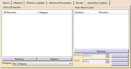
Go to the Geometry Creation tab.
-
Select the 3D elements (points or curves, including closed curves) to transfer to 2D.
You can transfer a point or a curve on a ply from 3D to 2D.
The 3D point or curve transferred on the 2D ply must lie on the same shell as the ply, otherwise the transfer cannot be done.
Only the part of the 3D curve lying on the ply is transferred on the 2D geometry.
When the segments exceed the ply contour, they are not taken into account. A contextual menu is available to create the elements.
Selected 3D elements are listed under 3D to 2D transfer, with the category applied to each element.- By default, the category is No Category.
- You can edit category on each ply.
-
Select 3D elements, sharing the same category or not.
-
Select a new category from the list.
The new category is applied to all selected 3D elements.
If you add 3D elements with no defined category, the last category you have selected is proposed by default.
You can edit it. -
Click Remove to remove selected elements from the elements to transfer.
-
To replace one 3D element:
- Select the 3D element to replace.
- Click Replace.
- Select an element to transfer.
It replaces the selected element unless it is already listed under 3D to 2D transfer. - Repeat on all the 3D elements to replace, one by one.
-
Click Preview.
The flattening is previewed on the plane tangent to the ply shell at the seed point. -
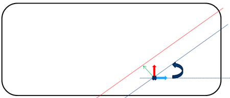
Enter the parameter values to define the Fiber Mesh Curves to keep.
- Distance: Offset value appied to the rotated curve to
build the result curve (green arrow).
It is initialized to half the material roll width of the ply: When creating cut-pieces using Multi-Add, the seed point is at the middle of the cut-piece. - Angle between the Warp vector and the result curve
(circular arrow).
- Distance: Offset value appied to the rotated curve to
build the result curve (green arrow).
-
Click
- Add to create a single curve.
- or Multi-Add: A first curve is created with the entered parameters, as well as all other possible curves using a distance modified by the material roll width.
The curves are listed under Fiber Mesh Curves.
To modify the parameters of a given curve:- Select its line in the list.
- Modify the distance or the angle and click Modify Values.
-
Click OK.
The producibility parameters are created or updated. - Fiber Mesh Curves are visible features, updated by their own build.
- Kept Fiber Mesh Curves are visible datum-like features (no update).
- 3Dto2D transfers and flatten contours are invisible datum-like features, updated by producibility build.
![]()