Adding an Analysis Case
After completing the thermal analysis, you now have the results of the temperature distribution in the pipe intersection. In this task you will add an Analysis Case to perform a two-step structural analysis using the results from the thermal analysis.
Switch to the Nonlinear Structural Analysis workbench by selecting Start>Analysis and Simulation>Nonlinear Structural Analysis from the main menu bar.
Select Insert>Nonlinear Structural Case from the menu bar.
Nonlinear Structural-Case-1 is created and appended to the specification tree.
Note: Nonlinear Structural-Case-1 is underlined in the specification tree, which indicates that it is now the current analysis case. This case will be modified when you add or edit step definitions, and it will be used for analysis submission. You can make an analysis case current by right-clicking on it and selecting Set As Current Case from the menu that appears.
Click the Pressure Load icon
 to add a pressure load to the current step. Select the six internal surfaces shown in Figure 3–8. In the Pressure dialog box, enter a value of 3.5E06 N/m2 for the pressure, and click OK.
Symbols representing the applied pressure are displayed on the geometry, and a Pressure object appears in the specification tree under the Loads objects set for the current step—the general static step in the new structural case.
Click the Clamp Boundary Condition icon
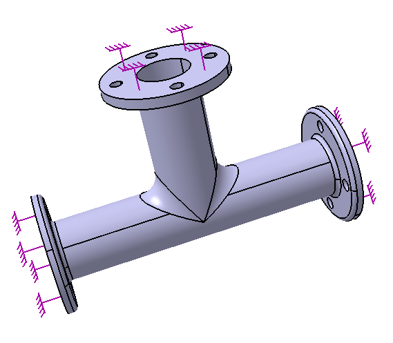
 . Select the three flange faces shown in Figure 3–11, and click OK in the Clamp BC dialog box.
A Clamp object appears in the specification tree under the Boundary Conditions objects set for the current step, and symbols appear on the selected faces indicating the constrained degrees of freedom.
Click the General Static Step icon
 to create a second step. In the General Static Step dialog box, enter a value of 200 seconds for the Step time, 20 seconds for the Initial increment size, and 200 seconds for the Maximum increment size. Accept the other default values, and click OK.
A second Static Step objects set appears in the specification tree under the Simulation History objects set for the current analysis case.
Note: The Static Step-2 object in the specification tree is now underlined, indicating that for the current analysis case, this is the step for which you are now defining loads and boundary conditions.
Click the Temperature History icon
 . Select the entire part by selecting the PartBody feature from the specification tree. In the Temperature History dialog box, select From job as the Distribution Type. Then select Job-1 in Thermal-Case-1 from the specification tree to identify the job from which the results should be read, and click OK.
Symbols representing the applied field are displayed on the geometry, and a Temperature History object appears in the specification tree under the Fields objects set for the current step.
Double-click the Job–2 feature located in the Jobs object set for Nonlinear Structural-Case-1 in the specification tree.
The Edit Job dialog box appears.
Enter a name and description for the job, accept the default values for the job data, and click OK.
Click the Job Manager icon
 , select the new job from the list in the Job Manager, and click Submit.
Click Continue in the Job Submission dialog box that appears with a list of informational consistency check messages.
When the analysis completes, click Attach Results in the Job Manager, and click OK in the dialog box that appears.
A link to the Abaqus output database file containing the results appears in the Links Manager, and two Static Step objects (one for each step) appear in the specification tree under the Analysis Case Solution feature.