Computing and Viewing Nodal Temperatures
In this task you will mesh the part, perform a thermal analysis, and create a plot of the nodal temperatures in the pipe intersection model.
Expand the Nodes and Elements feature in the specification tree, and double-click the OCTREE Tetrahedron Mesh.1 feature to edit the global characteristics of the mesh.
The OCTREE Tetrahedron Mesh dialog box appears.
In the OCTREE Tetrahedron Mesh dialog box, specify a global element Size of 0.05 m and a global element Absolute sag of 0.015 m. Accept the default choice of a linear element type, and click OK.
Right-click on the Nodes and Elements object in the specification tree, and select Mesh Visualization from the menu that appears.
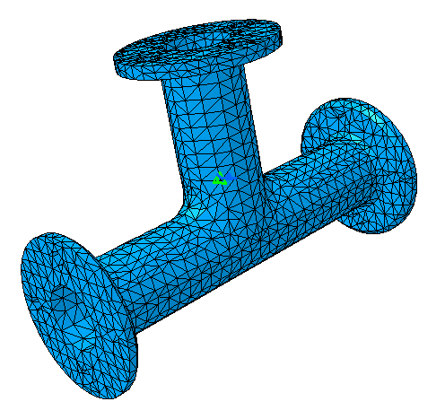
A warning message dialog box appears, informing you that the mesh needs to be updated; click OK to close the dialog box and to continue with the mesh generation. When the mesh generation is complete, the mesh is displayed on the part (see Figure 3–9) and a Mesh object appears under Nodes and Elements in the specification tree.
Expand the Jobs object set in the specification tree, and double-click the Job–1 feature to edit the analysis job.
The Edit Job dialog box appears.
Note: To create a new job for the current analysis case, click the Create Job icon
 .
.You can change the job identifier by editing the Name field. This name will be used in the specification tree and in the Job Manager.
Enter a description for the job in the Description field.
Accept the default values for the job data, and click OK.
Click the Job Manager icon
 .
.The Job Manager dialog box appears with a list of the jobs that you have created. By default, jobs for all Nonlinear and Thermal Analysis Cases are shown.
Select the job you created from the list in the Job Manager, and click Write Input.
By default, consistency checks are run when an input file is written. A Write Input File dialog box appears with the results of these consistency checks. In this case the Consistency Check Messages page lists the following message:
The Write Input File Messages tabbed page indicates that the input file was generated successfully.Feature Name Feature Type Message Severity Boundary Conditions/Heat Transfer Step-1 Boundary Condition Set Boundary condition set is empty Warning Click Close in the Write Input File dialog box.
The input file job name.inp is written to the specified computation directory for the job.
Click Submit in the Job Manager dialog box to submit the job to the Abaqus solver.
A Job Submission dialog box appears with the results of the consistency checks.
Since there have been no changes to the model since Abaqus for CATIA V5 wrote the input file, the results of the consistency checks are identical to those listed above. Click Continue.
Abaqus for CATIA V5 submits the job for analysis using the job settings defined in the job editor. The information in the Status column of the Job Manager updates to indicate the job's status. The Status column for this tutorial shows one of the following:
Submitted while the analysis input file is being generated.
Running while Abaqus analyzes the model.
Completed when the analysis is complete, and the output has been written to the output database file.
Aborted if Abaqus finds a problem with the input file or the analysis and aborts the analysis.
While the job is running, click Monitor in the Job Manager to monitor the progress of the analysis.
The job monitor dialog box appears. The top half of the dialog box displays the information available in the status (.sta) file that Abaqus/Standard creates for the job. The bottom half of the dialog box displays log file information, error and warning messages, and output information.
When the job completes successfully, click Close in the Job Monitor dialog box, and click Attach Results in the Job Manager.
A link to the Abaqus output database file containing the results appears in the Links Manager, and a Heat Transfer Step object appears in the specification tree under the Analysis Case Solution objects set for the current analysis case. In addition, the status of the Analysis Case Solution entry is updated to show that the solution is now available and is consistent with the model and history specification; in other words, the
 symbol no longer appears.
Plot the nodal temperatures.
Right-click on the Heat Transfer Step object under the Analysis Case Solution objects set in the specification tree, and select Generate Results Image from the menu that appears.
The Abaqus Image Generation dialog box appears with a list of the results available from the output database file for the specified step.
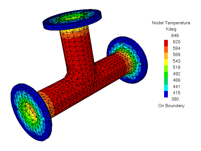
To plot contour values of nodal temperature for your model, select Nodal Temperature from the list of Available Images, and click OK.
The Abaqus Image Generation dialog box disappears, and the nodal temperatures are plotted on the model, as shown in Figure 3–10. A feature for the generated image appears under the Heat Transfer Step object in the specification tree.
Tip: You may need to hide the nodes and elements and change the render style to view the contour plot clearly. Right-click on the Nodes and Elements feature in the specification tree, and select Hide/Show from the menu that appears. To apply a render style to the part that reflects the material assignment, select View>Render Style>Customize View from the menu bar, and toggle on Materials in the Custom View Modes dialog box that appears.