Creating Smooth Step Amplitudes
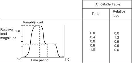
Smooth step amplitudes define the amplitude curve as a table of values at convenient points on the time scale with a smoothing algorithm applied near each of the points. Abaqus smooths the curve by setting the first and second derivatives to zero near each data point such that there is a smooth transition at each change in amplitude.
An example of a smooth amplitude is shown in Figure 11–2.
This task shows you how to create a smooth step amplitude.
Click the Smooth Step Amplitude icon
 .
.The Smooth Step Amplitude dialog box appears, and a Smooth Step Amplitude object appears in the specification tree under a Nonlinear and Thermal Properties feature.
You can change the identifier of the amplitude by editing the Name field.
Select the Time Span for the amplitude: Step Time or Total Time. Except for certain linear perturbation procedures, step time is measured from the beginning of each step. Total time starts at zero and is the total accumulated time over all general analysis steps within a particular analysis case; total time does not accumulate during linear perturbation steps.
Enter the time versus amplitude values into the table, or click the Folder icon
 to import the amplitude data from a text file. The amplitude magnitudes must be specified as multiples (fractions) of the reference magnitudes given for the load, boundary condition, or field.
Click OK in the Smooth Step Amplitude dialog box.