How are element stresses computed?
Element stresses at Gauss points are the product of the Comportment Law and the Strain Deformation.
|
|
-
 is the element stress
 -
 is the Comportment Law, computed as a function of the following
parameters, where:
is the Comportment Law, computed as a function of the following
parameters, where:-
 is the Poisson Ratio
 -
 is the Young's Modulus
-
-
 is the Strain deformation, computed according to the displacement.
For example, with a 2D displacement:

where
 and
and
 are the two partial derivatives.
How are contact elements computed?
-
It is assumed that contact property is non-linear (of the form K.X = F(X) ). Nevertheless, in the particular case of contact without friction, the solution is unique: it does not depend on the path used to put the two geometries in contact.
Static solutions inside the Generative Part Structural Analysis (GPS) product are thus solved with an iterative algorithm which could be qualified by an "advanced linear" approach. At each computation step, local contact directions are not updated (contrary to non-linear solvers). But if the local curvature is small (compared to contact area width), this approximation remains reliable and gives good results.
The contact connection mesh is done between overlapping surfaces at their initial position. The solver does not take into account large relative sliding between surfaces in contact. Contact condition is only valid for elements connected by the mesh part.
-
In case of contact with friction: after each contact iteration, the friction effects are computed and the contact computation is launched again.
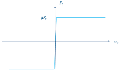
The computation uses a simplified Coulomb friction model.

The high slope near the y-axis is due to the initial high stiffness (not infinite).
Springs are added to keep the friction ratio small while maintaining contact. For the first iteration, there is no spring stiffness. The solver is started, and we determine Fc (contact force) and Dt (tangential displacement). The tangential stiffness Kt is added or updated.
The second iteration adds a high stiffness. Later iterations use Ft= Kt*Dt. If Ft > µ*Fc/Ft, test for convergence. If the solution is not converged, restart the solver and redetermine Fc and Dt.
-
To solve contact problems, an additional stiffness is added to the contact element.
Adding stiffness may influence displacements, especially in the case of two solids that are not really in contact.
For example: consider two surfaces (S1 and S2) with 2mm distance between.
Enforced displacements (dS1) are applied to S1: dS1 = -0.5mm.-
Case 1: (without contact)

In this case, the displacement of the S2 surface are dS2 = 0mm.
-
Case 2: (with contact)

where
 symbolizes the contact elements.
In this case dS2 is not equal to zero but the displacements are very small.
-
How are shell elements computed?
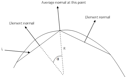
The average normal vector is used for shell elements.

where:
- L is the element length.
-
 is the angle between the element normal and the average normal.
 - R is the estimated curvature radius

When the angle between the element normal and the
average normal is smaller than the shell normal tolerance and if the ratio between the
curvature radius and the thickness is greater than two, the average
normal is used instead of the element normal for all the shell elements
(TR3, TR6, QD4, QD8).
The default value of the shell normal tolerance is 20 degrees and its
value can be set using the ELF_Shell_Normal_Tol environment
variable. See Singularity Computation.
How are node stresses computed?
Node stresses are extrapolations of element stresses.
The method consists in defining a continuous stress field within the element:
|
where:
|
These nodal stresses values are obtained using the least square minimization method:
|
where
|
How is error computed?
There are two steps in the error computation:
-
Stress smoothing.
This method consists in computing a weighted nodal stress value at each nodes.

For more information about the nodal stresses values, refer to How are node stresses computed?
-
Error estimation.
Once the nodal stresses values have been found, a continuous stress field is defined for each element:

where:
-
 are the element shape functions
 -
 are the smoothed nodal stresses

For more information about the nodal stresses values, refer to How are node stresses computed?
The error for each element (local error) is:

where:
-
 is the finite element solution field
 -
 is the Comportment Law

For more information about the nodal Comportment Law, refer to How are element stresses computed?
The total error (Estimated Precision) is the sum of all the local errors:

And the Global Estimated Error Rate is:

where
 is the global strain energy.
 -
How are result and computation files managed?
You can manage analysis results (contained in .CATAnalysisResults files) and analysis computations (contained in .CATAnalysisComputations files):
-
Specify the path of an external storage file directory.
For more details, refer to Specify External Storage. -
Clear Elfini Storage in order to save space on your disk.
For more details, refer to Clear External Storage. -
Specify a temporary data directory for the CATElfini stored data and computation results.
For more details, refer to Specify Temporary Data Directory.
You can also customize analysis default external storage
(computation and result data) settings.
For more details, refer to
External Storage.