|
-
Click Curvature Analysis
 in the Tools toolbar.
The Porcupine Curvature dialog box appears.
-
Click More...
The dialog box expands to reveal all its options. -
Select a curve in the work area.

In 2D Layout for 3D Design, select a curve in the active view of the work area. The curve is highlighted. A porcupine comb appears along the curve. The default type of this curve is Curvature.

You can
- Select multiple curves by sequentially selecting them in the 3D area.
- Select multiple curves at a time by trap selection.
- Select an already selected curve to clear its selection.
- Click in the empty space of the 3D area to clear every selection.
-
View the analysis on a curve:
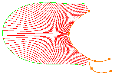
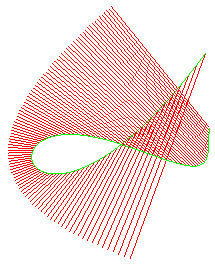
- In the Type area, select the type of analysis as Radius.
The porcupine comb shows the radius of the curve. - In the Type area, select the type of analysis as
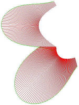
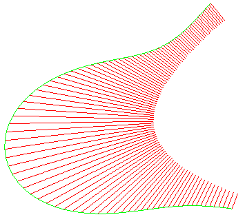
Curvature.
The porcupine comb shows the curvature of the curve.
Radius Analysis
 Curvature Analysis
For more information, see FreeStyle Shaper, Optimizer and Profiler User's guide: Basic Tasks: Analyzing curves and surfaces: Performing a Curvature Analysis.
- In the Type area, select the type of analysis as Radius.
- In the dialog box:
- Select Plane curves option.
This option projects the porcupine analysis on a mean plane, if it exists within the given tolerance. The minimum tolerance is 0.001mm.
The Tolerance box is available for edition. - Enter the required tolerance.
- Select Plane curves option.
- Define the amplitude characteristics of
porcupine comb.
- In the Amplitude
area, clear the
Automatic option.
When the Automatic amplitude check box is selected, the length of the spikes is optimized. So, even when zooming in or out, the spikes are always visible.
The Amplitude box is available for modification. - Click X 2.
The amplitude is doubled. - Click / 2.
The amplitude is halved. - Select the Logarithm
option.
The nature of the comb is changed to logarithmic. - Select the Reverse
option.
The porcupine comb is reversed. - Clear the Comb
option.
The envelope of the porcupine comb is visible, the teeth are not. - Clear the Envelop
option.
The teeth of porcupine comb are visible, the envelop is not.At a time, you must select either Comb, or Envelop options.
- In the Amplitude
area, clear the
Automatic option.
- Define the density characteristics of porcupine
comb.
- In the Density
area, define the density of the teeth in the comb.
Adjusting the density of the spikes is useful when the geometry is too dense to read but the resulting curve may not be smooth enough for analysis. - Click X 2.
The density is doubled. - Click / 2.
The density is halved. - Select the Curvilinear
option.
In the curvature graph, the X axis abscissa is curvilinear when Curvilinear is enabled, otherwise the X axis abscissa is parametric. When X axis abscissa is parametric, its range is not necessarily between zero and one. - Select the Particular
option.
The points of maximum and minimum magnitude are displayed on the curve.If you select both Particular and Project on Plane options, the inflection points are displayed over the comb. - Select the Inverse
option.
The inverse values in radius or curvature appear when the Curvature or Radius option are selected, respectively. This option does not recalculate maximum and minimum values. It only displays the inverse values. The maximum and minimum location for the selected type are still displayed.
- In the Density
area, define the density of the teeth in the comb.
- Right click on any tooth of the comb and select
Keep this point.
Point.x is listed in the tree.If you select the Particular option, then following contextual commands are available: - Keep this point
- Keep local minimum
- Keep local maximum
- Keep global minimum
- Keep global maximum
- Keep all minimum
- Keep all maximum
- View the curvature diagram:
- In the Diagram
area, select Display
diagram window
 .
.
The curvature amplitude and parameter of the analyzed curve are represented in this diagram.
The 2D Diagram dialog box appears. The color of the curves in the 2D Diagram dialog box match the ones on the geometry. - Move the cursor over the porcupine comb in the work
area.
The local amplitude is displayed in the work area and the current location is displayed in the 2D Diagram dialog box. - Right-click a curve in the
2D Diagram and choose one of the following
options:
- Drop marker: adds Points.x in the tree.
- Inverse X-coord
- Inverse Y-coord
- You can use the following options in
2D Diagram dialog box:
- All curves with the same vertical length
- All curves with the same origin
- Use a logarithmic scale on vertical axis
- More Options >>: The Diagram Options dialog box appears. With these options you can customize the 2D diagram viewing area.
- If you exit the Sketcher during sketch analysis and reopen the sketch within the same session, the analysis is resumed.
- In 2D Layout for 3D Design, the analysis is only visible for the geometrical elements in the current view. Changing the active view hides the analysis and shows it when the view is activated again. Similarly, the analysis is visible for geometrical elements in main view of the sheet. Changing the main view to background view hides the analysis.
- To stop the analysis, either click on the Curvature Analysis icon, or click in the empty space to unselect all the elements and then close the dialog box.
- The Quick Analysis tab in the Porcupine Curvature dialog box is only available in the Freestyle workbench.
- The following types of elements are
unavailable for selection, analysis, or
propagation:
- Construction elements
- Axis elements
- H and V elements
- Output features
- In the Diagram
area, select Display
diagram window
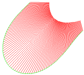
Auto-propagation of the porcupine comb
| The curve is in a connected profile. | The comb propagates along the
connected profile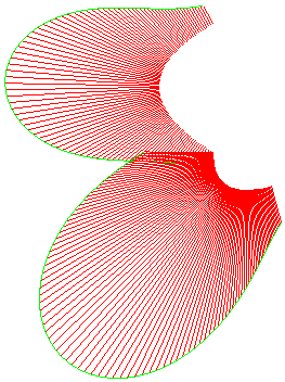 |
||
| The curve is in a connected profile posed to ambiguity. |
|
||
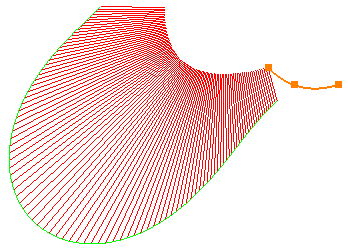
| The curve is in an unambiguous connected profile and initial element is removed. |
|